A couple years after “Attention is all you need” was published I had done some transformer training and inference. It was quite a leap in long range memory over RNNs like GRUs and LSTMs, which I played around with also. RNNs forget quickly and transformers are a dramatic improvement over them because of self-attention. Self-attention figures out how a long sequence of tokens work together and communicate with each other.
Self-Attention
Inference generates the next token based on a sequence of tokens. During inference, a sequence of tokens is attended to, to determine what information the current and previous tokens contribute to a new representation of the current token.
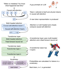 Training also learns by attending to current and previous tokens. A causal mask prevents a token from looking ahead to other tokens in the sequence during training. It’s important to not attend to future tokens during training because it’s impossible for the current token to attend to future tokens during inference.
During inference, when the current token is processed, three projections are made: Query, Key and Value. They are often described as:
Query is “What am I looking for?”
Key is “What information do I represent?”
Value is “Here’s the information I will provide.”
For current token’s vector t, the projections are calc’d like so:
Q = WQ × t

K = WK × t

V = WV × t
WQ, WK, and WV are weight matricies learned during training. K and V are cached for subsequent token processing.
The self-attention mechanism compares the current token’s Q to all the K’s in the sequence of tokens to create scores.
Q · K, ..., Q · K -> [score, ..., score] = scores
Softmax is applied to the scores to get attention weights.
softmax(scores) -> [weight, ..., weight] = attention weights
Attention weights are used to calc all the V’s contributions to the current token’s new representation.
wV + ... + wV -> [x, ..., x] = weighted sum vector
The weighted sum vector is the output representation of the currently processed token for a single head. A ‘head’ concentrates on token patterns and relationships. In language, words have all sorts of patterns and relationships, like subject-verb, word proximities, punctuation, semantics, syntax, and others. It’s helpful to think of an attention head being analogous understanding word relationships, though what each head learns is not easily transparent.
A transformer layer is muli-headed, and concats the representations from all heads, does a linear projection on that, then feeds that to a feed forward neural net. Transformer layers are stacked, and each layer builds on previous layers outputs, which helps build more complex token representations.
The stack’s last transformer layer outputs a final representation, which is an accumulation of the most important informaton about the current token and all its preceding tokens. The representation is used to calc logits that are converted to probabilities for a model’s token vocabulary. There could be tens of thousands of tokens or more in a vocabulary. One token is selected using probabilities to be the next token in the sequence.
Compute
How much processing does generative LLM inference need now? The transformer architecture has kept scaling up over time. For an idea of the magnitude, lets count ‘token visits’ needed by a decoder to generate a token these days. Full attention to a 1M token context, 64 heads, and 80 layer stack is:
1M x 64 x 80 = 5,120,000,000 token visits to generate one token! One!! It’s so mindblowing I’m adding this emoji here -> @_@.
That explains the electric bill, and why so much effort goes into:
– KV cache: quantization, sliding windows, GQA, paged attention
– Classification/routing: BERT, GLiClass, Jev, Kev, Laya
– MCP delegation